A Language Model for the Sky

Transformers ¹ were originally designed for language using sequences of tokens where each element attends to all the others to build up context. But weather is also a sequence problem. Every hour of temperature, humidity, wind speed, and cloud cover is a token, and all of the patterns that matter, the approaching storm system, the seasonal swing, the coastal fog rolling in at night,live in the relationships between those tokens across days and weeks of history.

For the final project of my Deep Learning course, I built two Transformer models for weather forecasting: a focused single-location baseline trained on 50 years of daily data from Corvallis, Oregon, and a more ambitious multi-location model trained on 5 years of hourly readings across 145 locations in the western United States. The goal was to see whether a Transformer could learn when certain weather happens and where by generalizing across the radically different climates of coastal Oregon all the way down to sunny Southern California all at once.

Two Models, Two Scales

The Single-Location Baseline

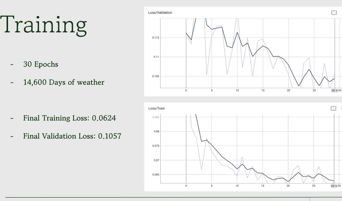
The first model is intentionally simple. Trained exclusively on weather data from Corvallis, Oregon spanning 1975 to 2025, it takes seven days of historical weather as context and predicts minimum temperature, maximum temperature, and weather type for the next day. The architecture is compact with two Transformer encoder blocks with 4 attention heads and an embedding dimension of 128 and it converges well, achieving a training loss of 0.0624 and a validation loss of 0.1057.

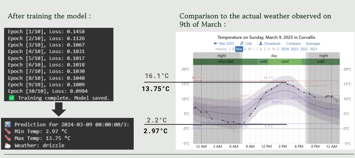
The Corvallis model is a proof of concept more than anything. It demonstrates that a Transformer can learn localized seasonal patterns with the wet Oregon winters, the dry summers, the shoulder seasons all from historical data alone. But a model that only works for one city isn’t very interesting. The harder question is whether you can train a single model that understands weather everywhere.

Multi-Location: The Real Challenge

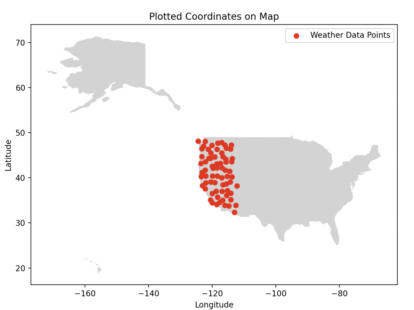
The multi-location model is substantially more complex. It was trained on 145 locations distributed across the western United States, with 5 years of hourly readings for 10 weather variables: temperature, rain, snowfall, humidity, wind speed, wind direction, sunshine duration, cloud cover, day/night indicator, and a categorical weather code. The sequence length is 168 hours, exactly one week, and the model predicts all 10 variables for the next hour simultaneously.

The architecture scales up accordingly: 6 Transformer encoder blocks, 8 attention heads, and separate prediction heads for each output variable. The categorical weather code (mapped from ~100 API values down to 10 meaningful categories like Clear Sky, Fog, Rain, Snow, Thunderstorm) gets its own embedding layer and a Cross-Entropy loss, while all the continuous variables use MSE. The losses are summed to update the weights in a single pass.

Training the multi-location model took 48 hours on an NVIDIA GPU on OSU’s HPC cluster and completed 20 epochs. A real reminder that Transformer models at this scale aren’t something you iterate on quickly.

Encoding Space and Time

The trickiest design problem in this project was representing where and when in a way the model could actually use.

Time is inherently circular, 11:59 PM is closer to midnight than 6:00 PM is, but if you encode the hour as a plain integer, the model sees 23 and 0 as maximally far apart. The fix is cyclical encoding: represent each time component as a sine/cosine pair, so the geometry of the encoding space matches the geometry of time. I applied this to hour of day, day of year, and month, as well as to wind direction (which has the same wraparound problem at 360°).

Location got the same treatment where latitude and longitude are encoded as sine/cosine pairs fed into the model as part of the input embedding. The idea was that nearby locations would have similar encodings, helping the model learn that coastal California and coastal Oregon share weather patterns that landlocked Nevada doesn’t.

In practice, this worked partially. The model learned broad regional trends well. But it struggled to hold onto location information over long sequences, which led to the most visible failure mode of locations that never see snow sometimes got snowfall predictions . The spatial encoding was only fed in at the first layer, and by the time the signal propagated through 6 Transformer blocks, the location context had effectively faded. My professor pointed out after the fact that injecting the location embedding at every layer, not just the input, would likely fix this. That’s a clear next step I didn’t have time to test.

What It Got Right, and What It Didn’t

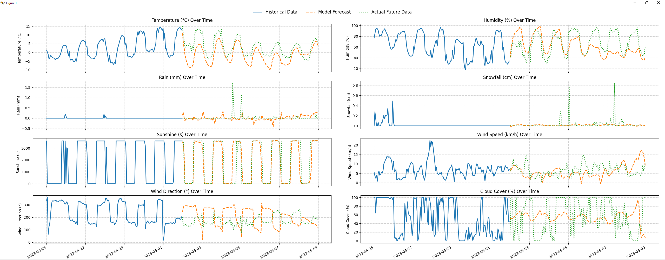
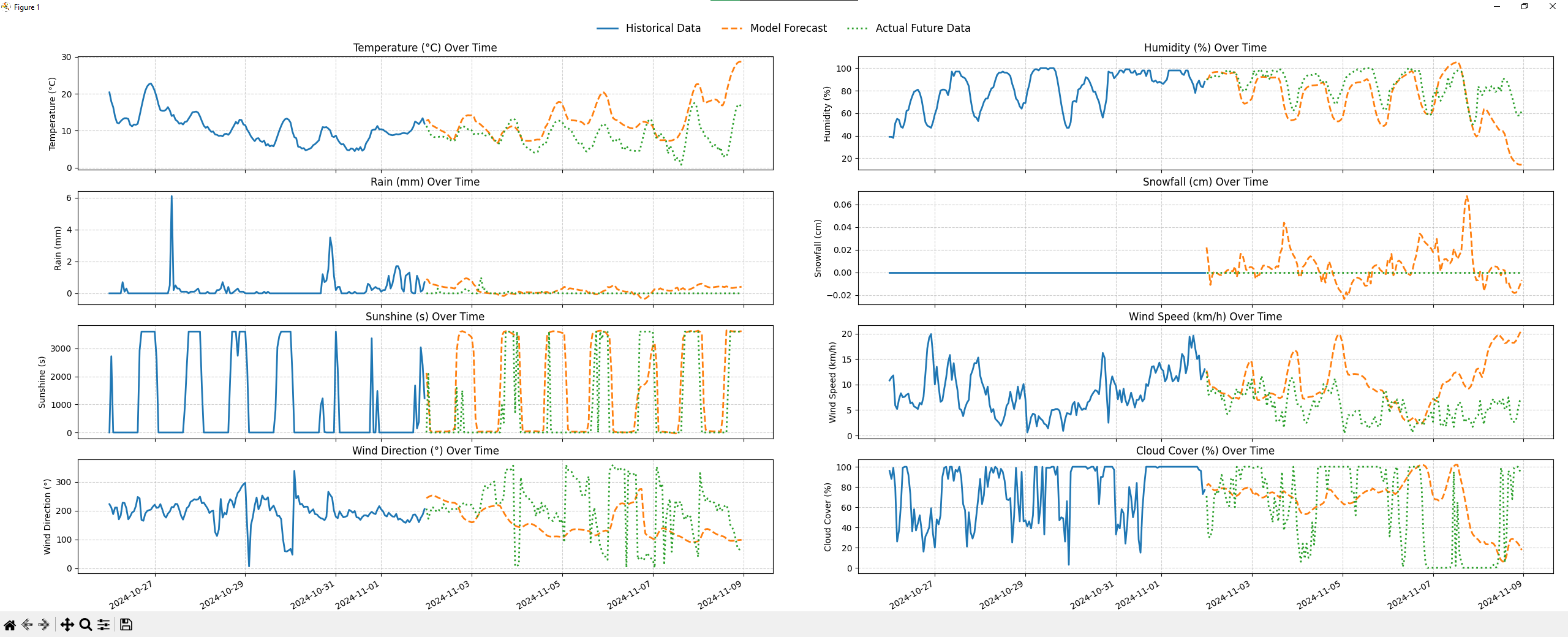
The honest assessment: the model is good at temperature trends, mediocre at precipitation, and unreliable on extremes.

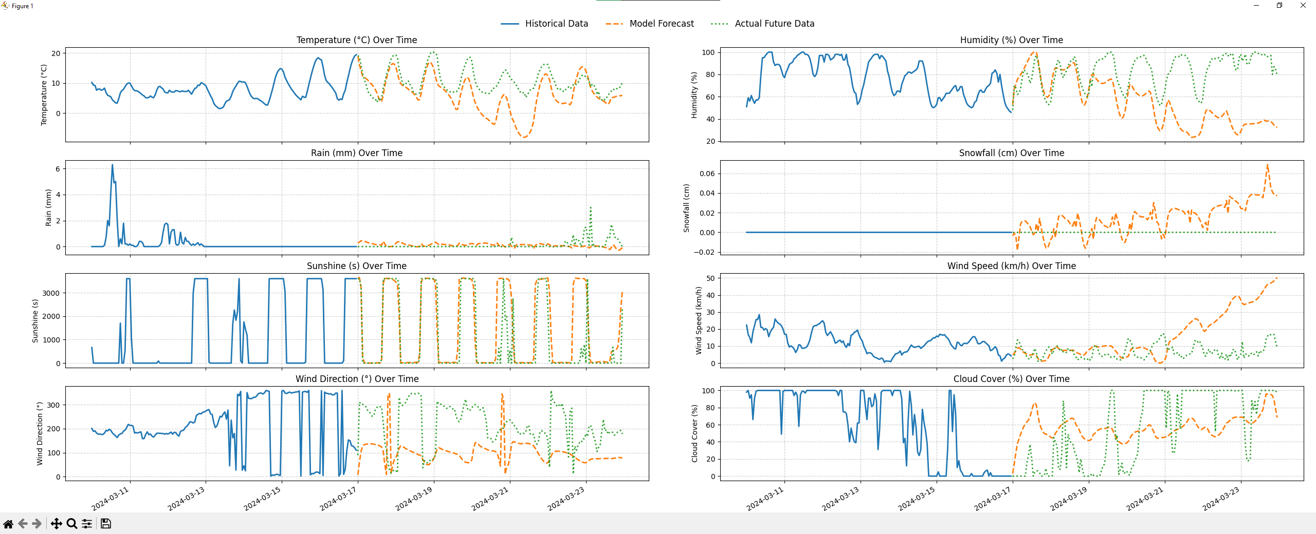
For temperature, the predicted trend lines closely track the actual future values for the first couple of days of the forecast window. Humidity follows reasonably well. But snowfall and rainfall, which are sparse and spiky by nature, are where the model struggles most. Rare events are hard to model because they appear infrequently in training data, and the model tends to over-predict precipitation at locations outside its training distribution.

There’s also a compounding error problem at longer horizons. The model predicts one hour at a time; for a 24-hour forecast, it feeds its own predictions back as context for subsequent steps. Each small error builds on the last, and accuracy degrades noticeably beyond the first few hours. This is a known challenge in autoregressive forecasting and isn’t unique to this model.

One genuinely interesting test was predicting at the geographically farthest point from any training location, the point inside the training region that is maximally distant from all 145 stations. The model still produced reasonable temperature predictions there, which suggests the spatial generalization is real, even if imperfect.

What I Learned

The most important lesson from this project is that honest evaluation is part of good ML work. It would have been easy to show only the predictions where the model looked great. Instead, you need to focus on the failures like the phantom snowfall, the degrading accuracy at longer horizons, the location-encoding limitation my professor identified. Those failures are more informative than the successes, and they point directly at what a future version of this model needs.

On the technical side, the most transferable insight is how much the encoding strategy matters for non-language sequence problems. Getting time and space into the right representational format by making it circular, normalized, injected at the right depth has an outsized effect on what the model can learn. The architecture itself was mostly standard and the interesting engineering was in the data preprocessing and the encoding design.

Key Contributions

• Designed and trained a single-location Transformer baseline on 50 years of daily weather data, achieving a validation loss of 0.1057
• Designed and trained a multi-location Transformer across 145 western US locations, predicting 10 simultaneous weather variables from 168-hour context windows
• Implemented cyclical temporal and spatial encodings for hour, day, month, wind direction, latitude, and longitude to preserve periodicity in the input representation
• Ran full training on OSU’s HPC cluster with CUDA GPU acceleration, monitored via Weights & Biases; multi-location model trained for 48 hours across 20 epochs
• Delivered the final class presentation solo after my partner was unable to contribute during finals week