Teaching a Neural Network to See Material Failure

When materials like graphite or carbon fiber are put under stress inside a Scanning Electron Microscope, researchers need to know exactly how and where the material is deforming at a pixel level. The standard tool for this is called Digital Image Correlation ¹ (DIC): a technique that divides an image into large square subsets and tracks where each region moves between frames. It works, but it has real limitations. Those subset boundaries lower the output resolution, noise creates false strain signals, and when a crack forms and breaks the assumption of smooth continuous motion, DIC can fail entirely and often right at the most scientifically interesting moment.

This is what our year-long senior capstone project set out to fix. Working directly with a faculty research partner, our team of six developed a full ML system to replace and augment DIC, producing per-pixel dense displacement fields from SEM image sequences. I served as both team lead and ML lead, owning the machine learning architecture and the synthetic data pipeline that made it all possible.

The Problem With Training Data

The first major challenge was the data. To train a neural network to estimate displacement between two SEM images, you need image pairs with known ground truth motion. Real SEM experiments don’t give you that. You can capture images before and after deformation, but you don’t know the true per-pixel displacement because that’s the thing you’re trying to predict.

The solution: generate it synthetically. Our faculty partner provided around 800 raw SEM image tiles of graphite microstructures. My job was to turn those 800 images into an effectively infinite training set with realistic, complex, ground-truth motion fields.

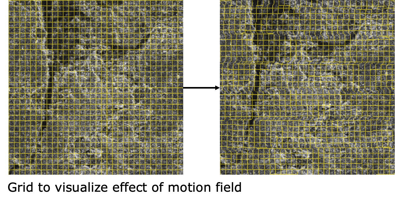
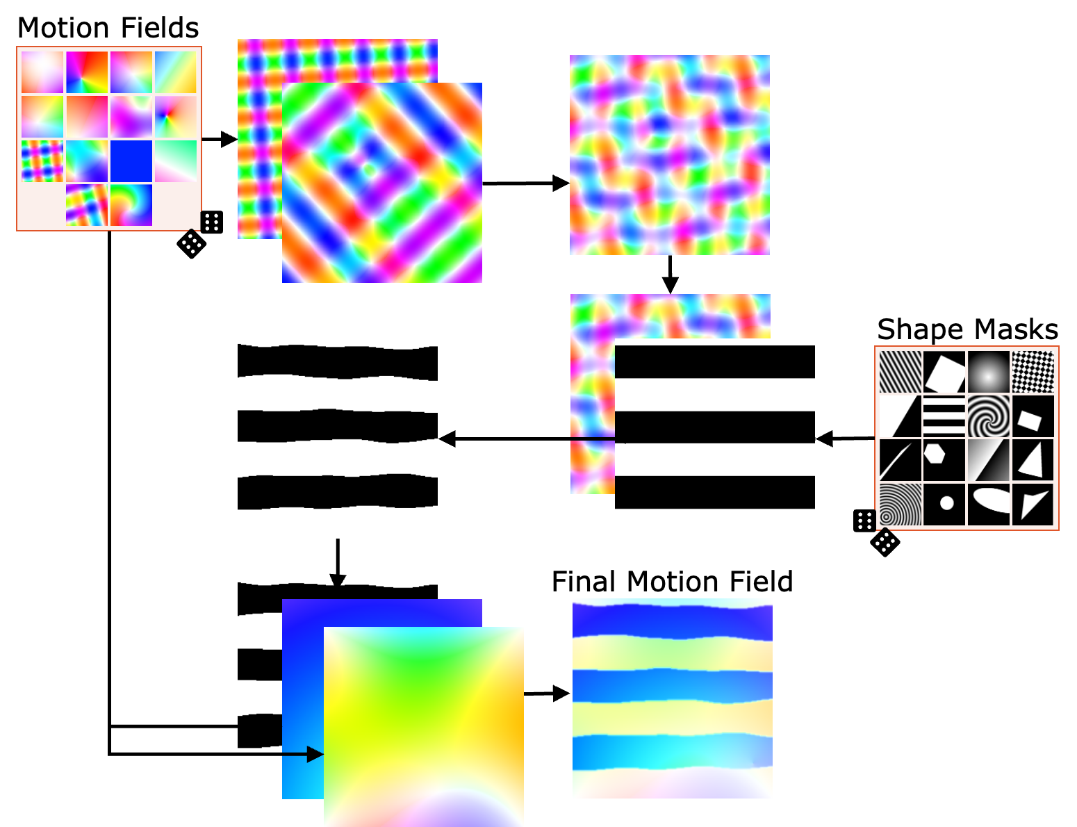
The pipeline works like this: for each training sample, take a real SEM tile as the reference image, generate a complex randomized vector displacement field, warp the reference image using that field to produce the deformed image, and use the field itself as the ground truth label. The model learns to predict the field from the image pair.

The vector field generation was the part I spent the most time on. Early attempts using simple global affine transformations such as translation, rotation, scaling and produced a model that looked decent on synthetic validation data but performed poorly on real SEM sequences. The problem was that real material deformation isn’t globally smooth. Near a crack, the displacement field has sharp, abrupt discontinuities where the material on one side of a crack moves completely independently from the other side. A model that had only ever seen smooth warps had no idea what to do with that.

The fix was a shape mask augmentation system. Applied with 75% probability per training sample, it works in several steps:

1. Generate a base displacement field from a random composition of harmonic warps, Perlin noise, swirl fields, and gradient fields
2. Randomly select a geometric mask, like a polygon, circle, grid, or procedural shape, and randomly position, scale, and rotate it
3. Warp the mask itself with a secondary displacement field so its edges aren’t geometrically perfect
4. Apply the mask by either inverting the base field inside the shape, or replacing it with an entirely new field thereby creating a sharp motion discontinuity at the boundary

This single addition was the biggest turning point in the project. After introducing shape masks, the model started correctly predicting localized displacement discontinuities at crack boundaries, which is exactly what DIC struggles most with. Over 82 epochs of training across multiple runs, the model was exposed to approximately 1,435,000 unique image pairs, all generated on-the-fly from those 800 base tiles by seeding the random generation from the epoch number and image index.

The Model Architecture

The neural network is a U-Net ² -based CNN, a well-established architecture for dense pixel-wise prediction tasks with a self-attention mechanism in the bottleneck.

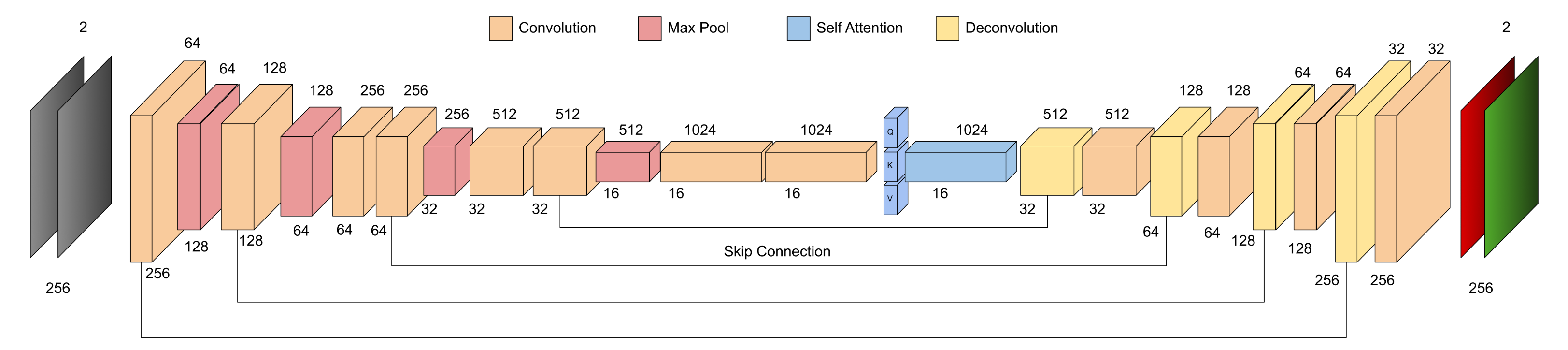
The network takes a stacked pair of 256×256 grayscale SEM images as input ([Batch, 2, 256, 256]) and outputs a 2-channel displacement field of the same size ([Batch, 2, 256, 256]), one channel for X displacement, one for Y. Every pixel gets its own motion vector.

The encoder progressively downsamples while doubling channel depth (64 → 128 → 256 → 512 → 1024), extracting increasingly abstract features. The decoder mirrors this symmetrically, using transposed convolutions to upsample back to full resolution, with skip connections carrying fine spatial detail from each encoder stage to its corresponding decoder stage. Every convolutional block includes a residual connection for gradient stability in the deep network.

The self-attention layer at the bottleneck was added because SEM deformation isn’t always local. A crack propagating across a frame creates correlated motion at locations that are far apart in pixel space. Attention lets the model build global context at the most compressed representation of the image, capturing those long-range dependencies that pure convolution misses. The attention is scaled by a learnable parameter γ initialized to zero so the network can gradually incorporate the attention signal over the course of training rather than being overwhelmed by it early on.

Training used the Adam optimizer ³ with an initial learning rate of 1×10⁻⁴, ReduceLROnPlateau ⁴ scheduling, and gradient clipping at a max L2 norm of 1.0. The loss function was End Point Error (EPE). The Euclidean distance between the predicted and ground truth displacement vector at each pixel which directly penalizes motion prediction errors without any assumptions about the relationship between neighboring pixels. Training ran on an NVIDIA Tesla V100-SXM3-32GB on OSU’s HPC cluster, with a batch size of 38 filling the 32GB of VRAM and four data loading workers to keep the GPU fed.

All training metrics were tracked and visualized in real-time using Weights & Biases ⁵ , which made it much easier to compare runs across different architectures and catch regressions early.

What The Model Actually Does Better

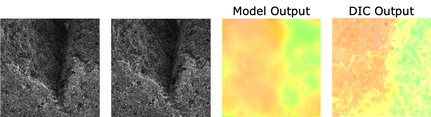
The core claim of this project is that a per-pixel dense displacement model outperforms DIC’s region-based approach. DIC outputs a displacement value per subset (typically a large square region). Our model outputs a displacement vector per pixel. The practical consequences of this difference are significant:

• Near cracks: DIC’s subsets straddle the crack boundary and fail, producing noise or exclusions. The ML model, trained on shape mask discontinuities, handles the boundary naturally
• Spatial resolution: DIC’s output resolution is limited by subset size. Our model produces full-resolution motion maps
• Noise robustness: The self-attention + skip connections let the model learn which image features indicate real motion versus sensor noise

One of the interesting evaluation findings (from my teammate’s frame gap analysis) was that the model is most accurate at small frame gaps (gap=1 or 2), where inter-frame displacement is small. At larger gaps (gap=10 to 20), prediction magnitude grows predictably because the model was primarily trained on small-motion examples and accumulates error as it tries to account for large jumps. This is a known limitation and a clear direction for future training data improvements.

The Full System

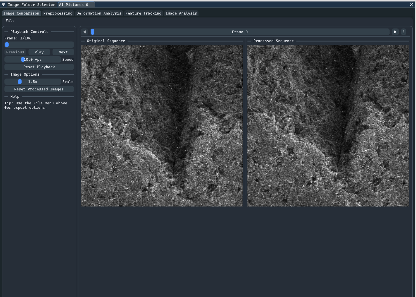
The ML model was my primary contribution, but the full deliverable was an integrated research tool. My teammate Adam built a comprehensive C++ GUI application that brought everything together: SEM image preprocessing, ML model inference, strain map visualization, and side-by-side DIC comparison. It also included a separate preprocessing GUI I developed earlier in the project for noise reduction and contrast enhancement using CLAHE.

The C++ application loaded our trained PyTorch ⁶ model via the C++ LibTorch ⁷ API and ran inference directly with no Python process or subprocess calls. Users could scrub through a SEM image sequence, adjust frame gap and tile overlap in real time, export displacement maps and strain GIFs, and compare the model’s output against DICe’s output on the same data.

The tool was delivered to Professor Tianyi Chen and his graduate student Spencer Doran, who tested it against their actual research data and provided the feedback that shaped many of the final features. By the project’s conclusion, it had been adopted for use in their ongoing research . This is the outcome we were most proud of.

Challenges and Learnings

The biggest technical challenge was the data diversity problem. Initial synthetic data used simple global warps, and the model trained on it couldn’t generalize to real crack behavior. The insight that solved it we could use shape masks for localized discontinuities, but it took several weeks of poor results before the root cause was clear. The lesson was when a model performs well on synthetic validation but poorly on real data, the gap is almost always in the training data distribution, not the architecture.

The other major challenge was a team dynamics one. One member was assigned critical ML evaluation and DICe comparison work that largely went unfulfilled, which meant I absorbed a significant portion of that work on top of my own. It made the last sprint brutal but ultimately pushed me to understand the full pipeline end-to-end in a way I wouldn’t have otherwise.

The project also changed direction significantly from its original scope of crack detection, strain prediction, and several other planned models were either simplified or dropped as we learned what was actually hard and what was actually useful. Being willing to let go of features that weren’t working and double down on what was became an important practice we adopted.

Key Contributions

• Designed and built the synthetic data generation pipeline, including the shape mask augmentation system, producing ~1.4M unique training samples from 800 base SEM images
• Architected and trained the U-Net + self-attention CNN for per-pixel dense displacement field estimation using PyTorch on OSU’s HPC cluster
• Managed all ML training and evaluation using Weights & Biases, iterating across architectures and parameters to optimize End Point Error
• Served as team lead, coordinating weekly goals, managing task allocation, and ensuring the project remained aligned with the research partner’s needs across the full year